Quickstart

This guide demonstrates JAX-bandflux with complete working examples. All code blocks are tested automatically to ensure they work with the current version.

SALT3 Light Curve Modeling

JAX-bandflux provides GPU-accelerated Type Ia supernova light curve modeling using the SALT3-NIR model.

Creating a SALT3 Source

The SALT3Source class provides the SALT3-NIR model with a functional API where parameters are passed as dictionaries:

import numpy as np
import jax
import jax.numpy as jnp
from jax_supernovae import SALT3Source, TimeSeriesSource
from jax_supernovae.bandpasses import get_bandpass
from jax_supernovae.salt3 import precompute_bandflux_bridge

source = SALT3Source()
print(source.param_names)

['x0', 'x1', 'c']

The SALT3 model has three parameters that describe the spectral time series:

• x0: Amplitude (overall flux normalization, typically 1e-5 to 1e-3)

• x1: Stretch (light curve width, typically -3 to 3)

• c: Color (dust-like reddening, typically -0.3 to 0.3)

The spectral flux density is given by: F(t, λ) = x₀ [M₀(t, λ) + x₁ M₁(t, λ)] × 10^(-0.4 CL(λ) c)

When fitting light curves, you also need t0 (time of peak) as a nuisance parameter, and redshift z which is typically fixed from spectroscopy.

Computing Bandflux

Calculate flux through a bandpass at a given phase (rest-frame days from peak):

params = {'x0': 1e-4, 'x1': 0.5, 'c': 0.05}
flux = source.bandflux(params, 'bessellb', 0.0, zp=27.5, zpsys='ab')
print(f"Flux at peak (B-band): {float(flux):.4e}")

Flux at peak (B-band): 6.2309e+02

Compute fluxes at multiple phases to see the light curve shape:

phases = np.array([-10.0, -5.0, 0.0, 5.0, 10.0, 15.0, 20.0])
fluxes = source.bandflux(params, 'bessellb', phases, zp=27.5, zpsys='ab')
for p, f in zip(phases, fluxes):
    print(f"  Phase {p:+5.1f} days: flux = {float(f):.2e}")

Phase -10.0 days: flux = 2.89e+02
Phase  -5.0 days: flux = 5.64e+02
Phase  +0.0 days: flux = 6.23e+02
Phase  +5.0 days: flux = 5.31e+02
Phase +10.0 days: flux = 3.89e+02
Phase +15.0 days: flux = 2.42e+02
Phase +20.0 days: flux = 1.47e+02

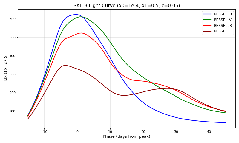
Plotting a Light Curve

Visualize the SALT3 light curve across multiple bands:

import matplotlib.pyplot as plt
import numpy as np
from jax_supernovae import SALT3Source

source = SALT3Source()
params = {'x0': 1e-4, 'x1': 0.5, 'c': 0.05}

# Generate light curve data
phases = np.linspace(-15, 45, 100)
bands = ['bessellb', 'bessellv', 'bessellr', 'besselli']
colors = ['blue', 'green', 'red', 'darkred']

plt.figure(figsize=(10, 6))
for band, color in zip(bands, colors):
    flux = source.bandflux(params, band, phases, zp=27.5, zpsys='ab')
    plt.plot(phases, np.array(flux), color=color, label=band.upper(), linewidth=2)

plt.xlabel('Phase (days from peak)', fontsize=12)
plt.ylabel('Flux (zp=27.5)', fontsize=12)
plt.title('SALT3 Light Curve (x0=1e-4, x1=0.5, c=0.05)', fontsize=14)
plt.legend(fontsize=11)
plt.grid(True, alpha=0.3)
plt.tight_layout()
plt.show()

Effect of SALT3 Parameters

See how x1 (stretch) affects the light curve:

print("Effect of x1 (stretch) on peak flux:")
for x1_val in [-2.0, -1.0, 0.0, 1.0, 2.0]:
    p = {'x0': 1e-4, 'x1': x1_val, 'c': 0.0}
    flux_peak = source.bandflux(p, 'bessellb', 0.0, zp=27.5, zpsys='ab')
    print(f"  x1 = {x1_val:+4.1f}: peak flux = {float(flux_peak):.2e}")

Effect of x1 (stretch) on peak flux:
  x1 = -2.0: peak flux = 6.25e+02
  x1 = -1.0: peak flux = 6.25e+02
  x1 = +0.0: peak flux = 6.24e+02
  x1 = +1.0: peak flux = 6.24e+02
  x1 = +2.0: peak flux = 6.23e+02

Generating Synthetic Data

For testing and development, generate synthetic supernova observations:

# True parameters for our synthetic supernova
TRUE_PARAMS = {'x0': 1.0e-4, 'x1': 0.5, 'c': 0.05}
TRUE_Z = 0.05  # Redshift
TRUE_T0 = 0.0  # Peak time

# Observation configuration
bands = ['bessellb', 'bessellv', 'bessellr']
obs_times = np.array([-10, -5, 0, 5, 10, 15, 20, 25, 30])

# Convert observer times to rest-frame phases
phases = (obs_times - TRUE_T0) / (1.0 + TRUE_Z)

# Generate observations for each band
np.random.seed(42)
all_times, all_fluxes, all_errors, all_bands = [], [], [], []

for band in bands:
    true_flux = np.array(source.bandflux(TRUE_PARAMS, band, phases, zp=27.5, zpsys='ab'))
    flux_err = np.abs(true_flux) * 0.05  # 5% errors
    noisy_flux = true_flux + np.random.normal(0, flux_err)
    all_times.extend(obs_times)
    all_fluxes.extend(noisy_flux)
    all_errors.extend(flux_err)
    all_bands.extend([band] * len(obs_times))

print(f"Generated {len(all_times)} observations across {len(bands)} bands")

Generated 27 observations across 3 bands

High-Performance Mode with Bridges

For likelihood evaluation in MCMC or nested sampling, pre-compute “bridges” for ~100x speedup:

# Convert to JAX arrays
times = jnp.array(all_times)
fluxes = jnp.array(all_fluxes)
fluxerrs = jnp.array(all_errors)

# Pre-compute bridges for each unique band
unique_bands = ['bessellb', 'bessellv', 'bessellr']
bridges = tuple(precompute_bandflux_bridge(get_bandpass(b)) for b in unique_bands)

# Map each observation to its band index
band_to_idx = {b: i for i, b in enumerate(unique_bands)}
band_indices = jnp.array([band_to_idx[b] for b in all_bands])

# Zero points for each observation
zps = jnp.full(len(times), 27.5)
print(f"Pre-computed {len(bridges)} bridges for bands: {unique_bands}")

Pre-computed 3 bridges for bands: ['bessellb', 'bessellv', 'bessellr']

Now compute model fluxes using the optimized path:

params = {'x0': 1e-4, 'x1': 0.5, 'c': 0.05}
model_fluxes = source.bandflux(
    params,
    bands=None,  # Use band_indices instead
    phases=times / (1 + TRUE_Z),
    zp=zps,
    zpsys='ab',
    band_indices=band_indices,
    bridges=bridges,
    unique_bands=unique_bands
)
print(f"Computed {len(model_fluxes)} model fluxes")

Computed 27 model fluxes

Defining a Likelihood Function

Create a JIT-compiled log-likelihood function for parameter estimation:

@jax.jit
def loglikelihood(x0, x1, c):
    """Gaussian log-likelihood for SALT3 parameters."""
    params = {'x0': x0, 'x1': x1, 'c': c}
    model = source.bandflux(
        params, None, times / (1 + TRUE_Z),
        zp=zps, zpsys='ab',
        band_indices=band_indices,
        bridges=bridges,
        unique_bands=unique_bands
    )
    chi2 = jnp.sum(((fluxes - model) / fluxerrs)**2)
    return -0.5 * chi2

# Evaluate at true parameters
logL_true = loglikelihood(1e-4, 0.5, 0.05)
print(f"Log-likelihood at true params: {float(logL_true):.2f}")

Log-likelihood at true params: -11.98

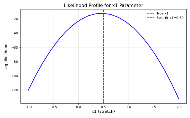
Finding the Best-Fit Parameters

Use a simple grid search to find optimal parameters:

# Grid search over x1 (stretch parameter)
x1_values = np.linspace(-1.0, 2.0, 21)
logL_values = [float(loglikelihood(1e-4, x1, 0.05)) for x1 in x1_values]

best_idx = np.argmax(logL_values)
best_x1 = x1_values[best_idx]
print(f"Best-fit x1: {best_x1:.2f} (true value: 0.50)")

Best-fit x1: 0.50 (true value: 0.50)

Plot the likelihood profile:

import matplotlib.pyplot as plt
import numpy as np
import jax.numpy as jnp
from jax_supernovae import SALT3Source
from jax_supernovae.bandpasses import get_bandpass
from jax_supernovae.salt3 import precompute_bandflux_bridge

# Generate synthetic data (same as doctest above)
TRUE_PARAMS = {'x0': 1.0e-4, 'x1': 0.5, 'c': 0.05}
TRUE_Z = 0.05
bands = ['bessellb', 'bessellv', 'bessellr']
obs_times = np.array([-10, -5, 0, 5, 10, 15, 20, 25, 30])
np.random.seed(42)

source = SALT3Source()
all_times, all_fluxes, all_errors, all_bands = [], [], [], []
for band in bands:
    phases = (obs_times - 0.0) / (1.0 + TRUE_Z)
    true_flux = np.array(source.bandflux(TRUE_PARAMS, band, phases, zp=27.5, zpsys='ab'))
    flux_err = np.abs(true_flux) * 0.05
    noisy_flux = true_flux + np.random.normal(0, flux_err)
    all_times.extend(obs_times)
    all_fluxes.extend(noisy_flux)
    all_errors.extend(flux_err)
    all_bands.extend([band] * len(obs_times))

times = jnp.array(all_times)
fluxes = jnp.array(all_fluxes)
fluxerrs = jnp.array(all_errors)
unique_bands = ['bessellb', 'bessellv', 'bessellr']
bridges = tuple(precompute_bandflux_bridge(get_bandpass(b)) for b in unique_bands)
band_to_idx = {b: i for i, b in enumerate(unique_bands)}
band_indices = jnp.array([band_to_idx[b] for b in all_bands])
zps = jnp.full(len(times), 27.5)

# Compute likelihood for different x1 values
x1_values = np.linspace(-1.0, 2.0, 21)
logL_values = []
for x1 in x1_values:
    params = {'x0': 1e-4, 'x1': x1, 'c': 0.05}
    model = source.bandflux(params, None, times / (1 + TRUE_Z),
                            zp=zps, zpsys='ab', band_indices=band_indices,
                            bridges=bridges, unique_bands=unique_bands)
    chi2 = float(jnp.sum(((fluxes - model) / fluxerrs)**2))
    logL_values.append(-0.5 * chi2)

best_idx = np.argmax(logL_values)
best_x1 = x1_values[best_idx]

plt.figure(figsize=(8, 5))
plt.plot(x1_values, logL_values, 'b-', linewidth=2)
plt.axvline(0.5, color='r', linestyle='--', label='True x1')
plt.axvline(best_x1, color='g', linestyle='--', label=f'Best-fit x1={best_x1:.2f}')
plt.xlabel('x1 (stretch)', fontsize=12)
plt.ylabel('Log-likelihood', fontsize=12)
plt.title('Likelihood Profile for x1 Parameter', fontsize=14)
plt.legend()
plt.grid(True, alpha=0.3)
plt.tight_layout()
plt.show()

For proper parameter estimation, see Sampling for nested sampling and optimization techniques.

Custom SED Models with TimeSeriesSource

For non-Type Ia supernovae or custom spectral models, use TimeSeriesSource:

# Define phase and wavelength grids
phase = np.linspace(-20, 50, 50)
wave = np.linspace(3000, 9000, 100)

# Create a simple Gaussian SED model
p_grid, w_grid = np.meshgrid(phase, wave, indexing='ij')
time_profile = np.exp(-0.5 * (p_grid / 12.0)**2)
wave_profile = np.exp(-0.5 * ((w_grid - 5500.0) / 1200.0)**2)
flux_grid = time_profile * wave_profile * 1e-15

# Create TimeSeriesSource
custom_source = TimeSeriesSource(
    phase, wave, flux_grid,
    zero_before=True,
    time_spline_degree=3,
    name='gaussian_sn'
)
print(custom_source.param_names)

['amplitude']

Compute bandflux with the custom model:

custom_params = {'amplitude': 2.5}
custom_flux = custom_source.bandflux(custom_params, 'bessellv', 0.0, zp=25.0, zpsys='ab')
print(f"Custom model flux at peak (V-band): {float(custom_flux):.4e}")

Custom model flux at peak (V-band): 6.5911e+03

For detailed TimeSeriesSource documentation, see TimeSeriesSource.

Next Steps

• API Differences from SNCosmo - Understand how JAX-bandflux differs from SNCosmo

• Data Loading - Load real supernova data

• Bandpass Loading - Work with astronomical filters

• Generating Model Fluxes - Advanced flux calculations

• Sampling - Parameter estimation with nested sampling