Generating Model Fluxes

This section explains how to calculate model fluxes using the SALT3 model in JAX-bandflux.

SALT3 Parameters

The SALT3 model is parameterized by the following variables:

Parameter	Typical Range	Description
`x0`	1e-6 to 1e-2	Amplitude (overall flux normalization)
`x1`	-3 to 3	Stretch (light curve width)
`c`	-0.3 to 0.3	Color (related to reddening)

Additionally, dust extinction can be applied using optional parameters:

dust_type: Integer index for the dust law (0=CCM89, 1=OD94, 2=F99)
ebv: E(B-V) reddening value
r_v: R_V parameter (default: 3.1)

Basic Flux Calculation

Create a SALT3Source and compute bandflux:

import numpy as np
import jax
import jax.numpy as jnp
from jax_supernovae import SALT3Source
from jax_supernovae.bandpasses import get_bandpass
from jax_supernovae.salt3 import precompute_bandflux_bridge

source = SALT3Source()
params = {'x0': 1e-4, 'x1': 0.5, 'c': 0.0}

# Single flux calculation at peak (phase=0)
flux = source.bandflux(params, 'bessellb', 0.0, zp=27.5, zpsys='ab')
print(f"B-band flux at peak: {float(flux):.4e}")

B-band flux at peak: 6.2401e+02

Multiple Phases

Compute flux at multiple phases (rest-frame days from peak):

phases = np.array([-10.0, -5.0, 0.0, 5.0, 10.0, 15.0, 20.0])
fluxes = source.bandflux(params, 'bessellb', phases, zp=27.5, zpsys='ab')
print("B-band light curve:")
for p, f in zip(phases, fluxes):
    print(f"  Phase {p:+6.1f}d: {float(f):8.2f}")

B-band light curve:
  Phase  -10.0d:   289.58
  Phase   -5.0d:   565.05
  Phase   +0.0d:   624.01
  Phase   +5.0d:   531.36
  Phase  +10.0d:   388.44
  Phase  +15.0d:   241.38
  Phase  +20.0d:   146.37

Multi-Band Flux Calculation

Compare flux across different bandpasses:

print("Flux at peak (phase=0) in different bands:")
for band in ['bessellb', 'bessellv', 'bessellr', 'besselli']:
    f = source.bandflux(params, band, 0.0, zp=27.5, zpsys='ab')
    print(f"  {band:10s}: {float(f):8.2f}")

Flux at peak (phase=0) in different bands:
  bessellb  :   624.01
  bessellv  :   579.78
  bessellr  :   484.52
  besselli  :   296.42

High-Performance Mode

For repeated calculations (MCMC, nested sampling), use pre-computed bridges:

# Pre-compute bridges
unique_bands = ['bessellb', 'bessellv', 'bessellr']
bridges = tuple(precompute_bandflux_bridge(get_bandpass(b))
                for b in unique_bands)

# Create observation data
n_obs = 21
phases = np.tile(np.linspace(-10, 30, 7), 3)  # 7 phases x 3 bands
band_names = ['bessellb'] * 7 + ['bessellv'] * 7 + ['bessellr'] * 7
band_to_idx = {b: i for i, b in enumerate(unique_bands)}
band_indices = jnp.array([band_to_idx[b] for b in band_names])
zps = jnp.full(n_obs, 27.5)

# Fast flux calculation
model_fluxes = source.bandflux(
    params, None, phases, zp=zps, zpsys='ab',
    band_indices=band_indices,
    bridges=bridges,
    unique_bands=unique_bands
)
print(f"Computed {len(model_fluxes)} fluxes in optimized mode")

Computed 21 fluxes in optimized mode

JIT-Compiled Flux Calculations

Wrap flux calculations in JIT-compiled functions for maximum speed:

@jax.jit
def compute_model(x0, x1, c, phases):
    params = {'x0': x0, 'x1': x1, 'c': c}
    return source.bandflux(
        params, None, phases, zp=zps, zpsys='ab',
        band_indices=band_indices,
        bridges=bridges,
        unique_bands=unique_bands
    )

model = compute_model(1e-4, 0.5, 0.0, phases)
print(f"JIT-compiled: computed {len(model)} fluxes")

JIT-compiled: computed 21 fluxes

Computing Chi-Squared

Calculate chi-squared statistic for model comparison:

# Simulate observed data with noise
np.random.seed(42)
true_fluxes = np.array(model_fluxes)
fluxerrs = np.abs(true_fluxes) * 0.05  # 5% errors
observed_fluxes = jnp.array(true_fluxes + np.random.normal(0, fluxerrs))
fluxerrs = jnp.array(fluxerrs)

# Chi-squared
chi2 = jnp.sum(((observed_fluxes - model_fluxes) / fluxerrs)**2)
print(f"Chi-squared: {float(chi2):.2f} for {len(model_fluxes)} data points")
print(f"Reduced chi-squared: {float(chi2)/len(model_fluxes):.2f}")

Chi-squared: 20.25 for 21 data points
Reduced chi-squared: 0.96

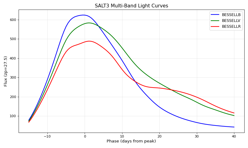
Light Curve Generation and Plotting

Generate a complete light curve across multiple bands:

import matplotlib.pyplot as plt

# Phase range
lc_phases = np.linspace(-15, 40, 100)

# Generate light curves for each band
print("Generating multi-band light curves...")
light_curves = {}
for band in ['bessellb', 'bessellv', 'bessellr']:
    fluxes = source.bandflux(params, band, lc_phases, zp=27.5, zpsys='ab')
    light_curves[band] = np.array(fluxes)
    peak_flux = np.max(fluxes)
    peak_phase = lc_phases[np.argmax(fluxes)]
    print(f"  {band}: peak flux = {float(peak_flux):.1f} at phase = {peak_phase:.1f}d")

Generating multi-band light curves...
  bessellb: peak flux = 624.3 at phase = -0.6d
  bessellv: peak flux = 583.5 at phase = 1.1d
  bessellr: peak flux = 488.8 at phase = 1.1d

Plot the light curves:

import matplotlib.pyplot as plt
import numpy as np
from jax_supernovae import SALT3Source

source = SALT3Source()
params = {'x0': 1e-4, 'x1': 0.5, 'c': 0.0}
lc_phases = np.linspace(-15, 40, 100)

plt.figure(figsize=(10, 6))
colors = {'bessellb': 'blue', 'bessellv': 'green', 'bessellr': 'red'}
for band in ['bessellb', 'bessellv', 'bessellr']:
    flux = source.bandflux(params, band, lc_phases, zp=27.5, zpsys='ab')
    plt.plot(lc_phases, np.array(flux), color=colors[band], label=band.upper(), lw=2)

plt.xlabel('Phase (days from peak)', fontsize=12)
plt.ylabel('Flux (zp=27.5)', fontsize=12)
plt.title('SALT3 Multi-Band Light Curves', fontsize=14)
plt.legend(fontsize=11)
plt.grid(True, alpha=0.3)
plt.tight_layout()
plt.show()

Parameter Effects on Light Curves

Explore how SALT3 parameters affect the light curve shape:

# Effect of color parameter (c)
print("Effect of color (c) on B-V color at peak:")
for c_val in [-0.2, -0.1, 0.0, 0.1, 0.2]:
    p = {'x0': 1e-4, 'x1': 0.0, 'c': c_val}
    flux_b = float(source.bandflux(p, 'bessellb', 0.0, zp=27.5, zpsys='ab'))
    flux_v = float(source.bandflux(p, 'bessellv', 0.0, zp=27.5, zpsys='ab'))
    # Convert to magnitudes
    mag_b = -2.5 * np.log10(flux_b) + 27.5
    mag_v = -2.5 * np.log10(flux_v) + 27.5
    bv_color = mag_b - mag_v
    print(f"  c = {c_val:+4.1f}: B-V = {bv_color:+.3f} mag")

Effect of color (c) on B-V color at peak:
  c = -0.2: B-V = -0.302 mag
  c = -0.1: B-V = -0.194 mag
  c = +0.0: B-V = -0.088 mag
  c = +0.1: B-V = +0.016 mag
  c = +0.2: B-V = +0.119 mag

Dust Extinction

JAX-bandflux supports three dust extinction laws:

CCM89: Cardelli, Clayton, Mathis (1989)
OD94: O’Donnell (1994)
F99: Fitzpatrick (1999)

To apply dust extinction, use the dust functions directly:

from jax_supernovae.dust import ccm89_extinction, apply_extinction

# Calculate extinction at given wavelengths
wavelengths = np.linspace(3000, 9000, 100)
ebv = 0.1
extinction = ccm89_extinction(wavelengths, ebv, r_v=3.1)

# Apply to flux
extincted_flux = apply_extinction(flux, extinction)

For dust parameters in SALT3 fitting, see the optimized_salt3_multiband_flux function which accepts dust parameters directly:

from jax_supernovae.salt3 import optimized_salt3_multiband_flux

params_with_dust = {
    'z': 0.05,
    't0': 0.0,
    'x0': 1e-4,
    'x1': 0.5,
    'c': 0.0,
    'dust_type': 0,  # CCM89
    'ebv': 0.1,
    'r_v': 3.1
}

model_fluxes = optimized_salt3_multiband_flux(
    times, bridges, params_with_dust, zps=zps, zpsys='ab'
)

For more details on dust extinction, see Dust Extinction.

Redshift Handling

SALT3 models rest-frame spectra. Convert observer-frame times to rest-frame phases:

# Observer-frame times (MJD)
t0 = 58650.0  # Peak time
z = 0.05      # Redshift
observer_times = np.array([58640, 58650, 58660, 58670])

# Convert to rest-frame phases
rest_phases = (observer_times - t0) / (1 + z)
print("Time dilation effect:")
for t_obs, p_rest in zip(observer_times, rest_phases):
    print(f"  Observer MJD {t_obs}: rest-frame phase = {p_rest:+.2f} days")

Time dilation effect:
  Observer MJD 58640: rest-frame phase = -9.52 days
  Observer MJD 58650: rest-frame phase = +0.00 days
  Observer MJD 58660: rest-frame phase = +9.52 days
  Observer MJD 58670: rest-frame phase = +19.05 days

The redshift affects both the time dilation and the wavelength shift of the bandpass transmission.

Model Bounds

Check the valid range for your model:

print(f"Phase range: {source.minphase()} to {source.maxphase()} days")
print(f"Wavelength range: {source.minwave()} to {source.maxwave()} Angstroms")

Phase range: -20.0 to 50.0 days
Wavelength range: 2000.0 to 20000.0 Angstroms

Extrapolation outside these bounds may produce unreliable results.