TimeSeriesSource
TimeSeriesSource is a JAX-bandflux class for fitting custom supernova
spectral energy distributions (SEDs). It provides a JAX/GPU-accelerated
implementation matching sncosmo’s TimeSeriesSource API whilst using a
functional parameter-passing approach for optimal performance in MCMC and
nested sampling applications.
Key Features
Custom SED Models: Fit any spectral time series defined on a 2D (phase × wavelength) grid
Bicubic Interpolation: Matches sncosmo exactly using JAX primitives
Functional API: Parameters passed as dictionaries for JAX compatibility
Two-Tier Performance: Simple mode for convenience, optimised mode for speed
JIT Compatible: Works seamlessly in JIT-compiled likelihood functions
GPU Accelerated: Runs efficiently on GPUs via JAX
Numerical Accuracy: Matches sncosmo to <0.01% (tested)
API Comparison: sncosmo vs JAX-bandflux
Constructor (Nearly Identical)
sncosmo:
source = sncosmo.TimeSeriesSource(phase, wave, flux,
                                   zero_before=False,
                                   time_spline_degree=3,
                                   name=None, version=None)
JAX-bandflux:
source = TimeSeriesSource(phase, wave, flux,  # Same signature!
                          zero_before=False,
                          time_spline_degree=3,
                          name=None, version=None)
Method Calls (Functional API)
sncosmo (stateful):
source.set(amplitude=1.0)
flux = source.bandflux('bessellb', 0.0, zp=25.0, zpsys='ab')
JAX-bandflux (functional):
params = {'amplitude': 1.0}
flux = source.bandflux(params, 'bessellb', 0.0, zp=25.0, zpsys='ab')
The key difference: JAX-bandflux passes parameters as a dictionary to each method call, enabling JAX to trace parameter dependencies for autodiff and JIT compilation.
Basic Usage
Creating a TimeSeriesSource
# Define your model grid
phase = np.linspace(-20, 50, 100)  # Days
wave = np.linspace(3000, 9000, 200)  # Angstroms

# Create flux array (phase × wavelength)
p_grid, w_grid = np.meshgrid(phase, wave, indexing='ij')
time_profile = np.exp(-0.5 * (p_grid / 12.0)**2)
wave_profile = np.exp(-0.5 * ((w_grid - 5500.0) / 1200.0)**2)
flux_grid = time_profile * wave_profile * 1e-15

# Create source
source = TimeSeriesSource(phase, wave, flux_grid,
                          zero_before=False,
                          time_spline_degree=3,
                          name='my_model')
print(source.param_names)
['amplitude']
Simple Photometry
# Define parameters
params = {'amplitude': 1.0}

# Single observation at peak (phase=0)
flux_b = source.bandflux(params, 'bessellb', 0.0, zp=25.0, zpsys='ab')
print(f"B-band flux at peak: {float(flux_b):.4e}")

# Light curve (multiple phases, same band)
phases = np.linspace(-10, 30, 10)
fluxes_b = source.bandflux(params, 'bessellb', phases, zp=25.0, zpsys='ab')
print("B-band light curve:")
for p, f in zip(phases[:5], fluxes_b[:5]):  # Show first 5
    print(f"  Phase {p:+6.1f}d: {float(f):8.2f}")

# Multi-band observation (same phase, different bands)
bands = ['bessellb', 'bessellv', 'bessellr']
phases_same = np.zeros(3)
fluxes_multi = source.bandflux(params, bands, phases_same, zp=25.0, zpsys='ab')
print("Flux at peak in different bands:")
for band, flux in zip(bands, fluxes_multi):
    print(f"  {band:10s}: {float(flux):8.2f}")
B-band flux at peak: 1.1498e+03
B-band light curve:
  Phase  -10.0d:   812.49
  Phase   -5.6d:  1032.93
  Phase   -1.1d:  1144.86
  Phase   +3.3d:  1106.27
  Phase   +7.8d:   931.95
Flux at peak in different bands:
  bessellb  :  1149.78
  bessellv  :  2636.44
  bessellr  :  2538.65
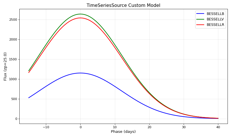
Plotting a Custom Model Light Curve
Visualize the custom SED model across multiple bands:
import matplotlib.pyplot as plt
import numpy as np
from jax_supernovae import TimeSeriesSource

# Create custom SED model
phase = np.linspace(-20, 50, 100)
wave = np.linspace(3000, 9000, 200)
p_grid, w_grid = np.meshgrid(phase, wave, indexing='ij')
time_profile = np.exp(-0.5 * (p_grid / 12.0)**2)
wave_profile = np.exp(-0.5 * ((w_grid - 5500.0) / 1200.0)**2)
flux_grid = time_profile * wave_profile * 1e-15

source = TimeSeriesSource(phase, wave, flux_grid,
                          zero_before=False,
                          time_spline_degree=3,
                          name='my_model')
params = {'amplitude': 1.0}

# Generate light curve data
lc_phases = np.linspace(-15, 40, 100)
bands_plot = ['bessellb', 'bessellv', 'bessellr']
colors = {'bessellb': 'blue', 'bessellv': 'green', 'bessellr': 'red'}

plt.figure(figsize=(10, 6))
for band in bands_plot:
    flux = source.bandflux(params, band, lc_phases, zp=25.0, zpsys='ab')
    plt.plot(lc_phases, np.array(flux), color=colors[band], label=band.upper(), linewidth=2)

plt.xlabel('Phase (days)', fontsize=12)
plt.ylabel('Flux (zp=25.0)', fontsize=12)
plt.title('TimeSeriesSource Custom Model', fontsize=14)
plt.legend(fontsize=11)
plt.grid(True, alpha=0.3)
plt.tight_layout()
plt.show()
Calculate Magnitudes
# Magnitude in AB system
mag_b = source.bandmag(params, 'bessellb', 'ab', 0.0)
print(f"B-band magnitude at peak: {float(mag_b):.2f} mag")

# Multi-band magnitudes
print("Magnitudes at peak:")
for band in ['bessellb', 'bessellv', 'bessellr']:
    mag = source.bandmag(params, band, 'ab', 0.0)
    print(f"  {band:10s}: {float(mag):.2f} mag")
B-band magnitude at peak: 17.35 mag
Magnitudes at peak:
  bessellb  : 17.35 mag
  bessellv  : 16.45 mag
  bessellr  : 16.49 mag
High-Performance Mode
For MCMC, nested sampling, or any application requiring many model evaluations, use the optimised mode with pre-computed bridges:
# Example: 30 observations in 3 bands
n_obs = 30
obs_phases = np.linspace(-10, 40, n_obs)
band_names = ['bessellb', 'bessellv', 'bessellr'] * (n_obs // 3)
zps = jnp.ones(n_obs) * 25.0

# Pre-compute bridges ONCE (outside the likelihood)
unique_bands = ['bessellb', 'bessellv', 'bessellr']
bridges = tuple(precompute_bandflux_bridge(get_bandpass(b))
                for b in unique_bands)

# Create band indices mapping each observation to its bridge
band_to_idx = {'bessellb': 0, 'bessellv': 1, 'bessellr': 2}
band_indices = jnp.array([band_to_idx[b] for b in band_names])

# Fast calculation (10-100x faster than simple mode)
params = {'amplitude': 1.0}
fluxes = source.bandflux(params, None, obs_phases,
                         zp=zps, zpsys='ab',
                         band_indices=band_indices,
                         bridges=bridges,
                         unique_bands=unique_bands)
print(f"Computed {len(fluxes)} fluxes using optimized mode")
print(f"Mean flux: {float(jnp.mean(fluxes)):.2e}, range: [{float(jnp.min(fluxes)):.2e}, {float(jnp.max(fluxes)):.2e}]")
Computed 30 fluxes using optimized mode
Mean flux: 9.92e+02, range: [9.81e+00, 2.60e+03]
JIT-Compiled Likelihood Functions
TimeSeriesSource works seamlessly in JIT-compiled functions:
# Generate synthetic data
true_amplitude = 2.0
np.random.seed(123)
true_fluxes = np.array(source.bandflux({'amplitude': true_amplitude}, None, obs_phases,
                                       zp=zps, zpsys='ab',
                                       band_indices=band_indices,
                                       bridges=bridges,
                                       unique_bands=unique_bands))
flux_errors = np.abs(true_fluxes) * 0.05
observed_fluxes = jnp.array(true_fluxes + np.random.normal(0, flux_errors))
flux_errors = jnp.array(flux_errors)

# Define JIT-compiled likelihood
@jax.jit
def loglikelihood(amplitude):
    """Calculate log-likelihood for given amplitude."""
    params = {'amplitude': amplitude}
    model_fluxes = source.bandflux(params, None, obs_phases,
                                   zp=zps, zpsys='ab',
                                   band_indices=band_indices,
                                   bridges=bridges,
                                   unique_bands=unique_bands)
    chi2 = jnp.sum(((observed_fluxes - model_fluxes) / flux_errors)**2)
    return -0.5 * chi2

# Evaluate likelihood at true amplitude
logL_true = loglikelihood(2.0)
print(f"Log-likelihood at true amplitude (2.0): {float(logL_true):.2f}")

# Test at wrong amplitude
logL_wrong = loglikelihood(1.0)
print(f"Log-likelihood at wrong amplitude (1.0): {float(logL_wrong):.2f}")

print(f"Difference in log-likelihood: {float(logL_true - logL_wrong):.1f}")
Log-likelihood at true amplitude (2.0): -20.47
Log-likelihood at wrong amplitude (1.0): -1533.88
Difference in log-likelihood: 1513.4
Parameters
Constructor Parameters
Parameter |
Type |
Default |
Description |
|---|---|---|---|
|
array_like |
Required |
1D array of phase values (days). Must be sorted ascending. |
|
array_like |
Required |
1D array of wavelength values (Å). Must be sorted ascending. |
|
array_like |
Required |
2D array of flux values (erg/s/cm²/Å). Shape: (len(phase), len(wave)). |
|
bool |
False |
If True, flux is zero for phase < minphase. If False, extrapolates. |
|
int |
3 |
Time interpolation degree: 1 (linear) or 3 (cubic). |
|
str |
None |
Optional name for the model. |
|
str |
None |
Optional version identifier. |
Model Parameters (Functional API)
The functional API requires passing parameters as a dictionary to each method call:
Parameter |
Type |
Description |
|---|---|---|
|
float |
Scaling factor for the model flux. |
Example:
params = {'amplitude': 1.5}
flux = source.bandflux(params, 'bessellb', 0.0, zp=25.0, zpsys='ab')
print(f"Flux with amplitude=1.5: {float(flux):.2f}")

# Compare to amplitude=1.0
flux_1 = source.bandflux({'amplitude': 1.0}, 'bessellb', 0.0, zp=25.0, zpsys='ab')
print(f"Ratio: {float(flux / flux_1):.2f} (expected: 1.5)")
Flux with amplitude=1.5: 1724.67
Ratio: 1.50 (expected: 1.5)
Methods
bandflux
Calculate bandflux through specified bandpass(es).
Signature:
bandflux(params, bands, phases, zp=None, zpsys=None, **kwargs)
Parameters:
params(dict): Must contain'amplitude'bands(str, list, or None): Bandpass name(s). Use None for optimised mode.phases(float or array): Rest-frame phase(s) in dayszp(float or array, optional): Zero point(s)zpsys(str, optional): Zero point system (‘ab’, etc.)band_indices(array, optional): For optimised modebridges(tuple, optional): For optimised modeunique_bands(list, optional): For optimised mode
Returns:
float or array: Bandflux value(s) matching input shape
bandmag
Calculate magnitude through specified bandpass(es).
Signature:
bandmag(params, bands, magsys, phases, **kwargs)
Parameters:
params(dict): Must contain'amplitude'bands(str or list): Bandpass name(s)magsys(str): Magnitude system (‘ab’, etc.)phases(float or array): Rest-frame phase(s)Additional kwargs for optimised mode
Returns:
float or array: Magnitude value(s). Returns NaN for flux ≤ 0.
Properties
param_names: List of parameter names ([‘amplitude’])minphase(): Minimum phase of model (days)maxphase(): Maximum phase of model (days)minwave(): Minimum wavelength of model (Å)maxwave(): Maximum wavelength of model (Å)
Advanced Topics
Interpolation Methods
TimeSeriesSource supports two interpolation methods:
Cubic Interpolation (default):
source = TimeSeriesSource(phase, wave, flux, time_spline_degree=3)
Uses bicubic interpolation (same as sncosmo)
Smooth light curves
Better for well-sampled grids
Linear Interpolation:
source = TimeSeriesSource(phase, wave, flux, time_spline_degree=1)
Uses bilinear interpolation
Faster computation
Better for coarse grids or performance-critical applications
Zero-Before Behaviour
zero_before=False (default):
Extrapolates flux for phases before
minphaseUses edge values from the grid
Suitable for models where early-time flux is uncertain
zero_before=True:
source = TimeSeriesSource(phase, wave, flux, zero_before=True)
Returns exactly zero for phase <
minphaseSuitable for models that should not have flux before explosion
Matches sncosmo’s behaviour
Handling Redshift
TimeSeriesSource works in rest-frame. Calculate rest-frame phases outside:
z = 0.5
t0 = 58650.0
times_obs = np.array([58640, 58650, 58660, 58670])
phases_rest = (times_obs - t0) / (1 + z)
print(phases_rest)
[-6.66666667 0. 6.66666667 13.33333333]
Performance Tips
Use Optimised Mode for Fitting: Pre-compute bridges once, reuse many times
JIT Compile Likelihood Functions: Use
@jax.jitfor 10-100x speedupBatch Observations: Process multiple observations together when possible
Appropriate Grid Resolution: Balance accuracy vs memory/compute
Use GPU When Available: JAX automatically uses GPU if available
Comparison with SALT3Source
Feature |
TimeSeriesSource |
SALT3Source |
|---|---|---|
Model Type |
Custom SED |
SALT3-NIR only |
Parameters |
amplitude |
x0, x1, c |
Flexibility |
Any 2D flux grid |
Fixed SALT3 model |
Use Case |
Custom models, rare events |
Type Ia SNe standardisation |
Performance |
Comparable |
Comparable |
Both classes coexist and can be used together in the same analysis.
Common Issues
Q: Why does my model return NaN?
Check that:
Your phase/wavelength ranges cover the requested observations
Flux values are finite (no NaN/Inf in input grid)
For magnitudes: flux must be positive
Q: Why is simple mode slow?
Simple mode creates bandpass bridges on-the-fly. For repeated calculations (MCMC/nested sampling), use optimised mode with pre-computed bridges.
Q: Can I use this with nested sampling?
Yes! TimeSeriesSource is designed for this. Use optimised mode with the JIT-compiled likelihood pattern shown above. See Sampling for complete nested sampling examples.